Implementing Imitation Learning algorithms for CartPole
Table of Contents
- Introduction
- Behavior Cloning
- Alternating Optimization
- DAgger (Dataset Aggregation)
- Conclusion
- Resources
Introduction
Recently, I’ve been studying a subfield of RL called Imitation Learning, which I find fascinating due to its alternative approach to the central problem in RL. Usually in RL, an agent learns its behavior by interacting with the environment - that is, taking actions and collecting rewards. By contrast, in Imitation Learning the focus is on something completely different: you assume the existence of an expert agent, and train your agent to solely imitate that expert. In other words, you don’t want to create an AI that paints well; you want to create an AI that can imitate someone that paints well.

At first, the assumption of an expert might make Imitation Learning sound stupid (isn’t having the expert the whole problem?), but in practice, there are a ton of situations where having an expert is actually plausible:
- You want a robot to execute a certain manual task after watching a human demonstration (e.g. picking a block and placing it upside down);
- You want an agent to learn a game after watching footage of other people playing it;
- You have a black-box expert agent (e.g. a Deep Learning model) and you want to turn it into a transparent white-box agent (e.g. a Decision Tree agent).
I am particularly interested in that last point: to create interpretable agents by leveraging accurate and uninterpretable Deep Learning models. For that reason, I will assume that we have access to the expert at any time, which is not an assumption that we can always make (sometimes you just have a fixed number of demonstrations and that’s it). This specific problem is often called active imitation learning, and in this post I will explore three of the most popular approaches of this sort, alongside some implementations of my own. At the end of the page you’ll find links to the resources that I used.
Environment
In this post, we’ll use the OpenAI CartPole environment (also called inverted pendulum problem) as a running example. In this task, the goal is to move the cart left and right in order to keep a pole rightly balanced in the middle. The reward is +1 for each timestep the pole is balanced, up to a maximum of 500 timesteps. The environment has 4 different attributes: cart position, cart velocity, pole angle and pole angular velocity. This environment is not difficult at all, but I think it serves as a good visual example.
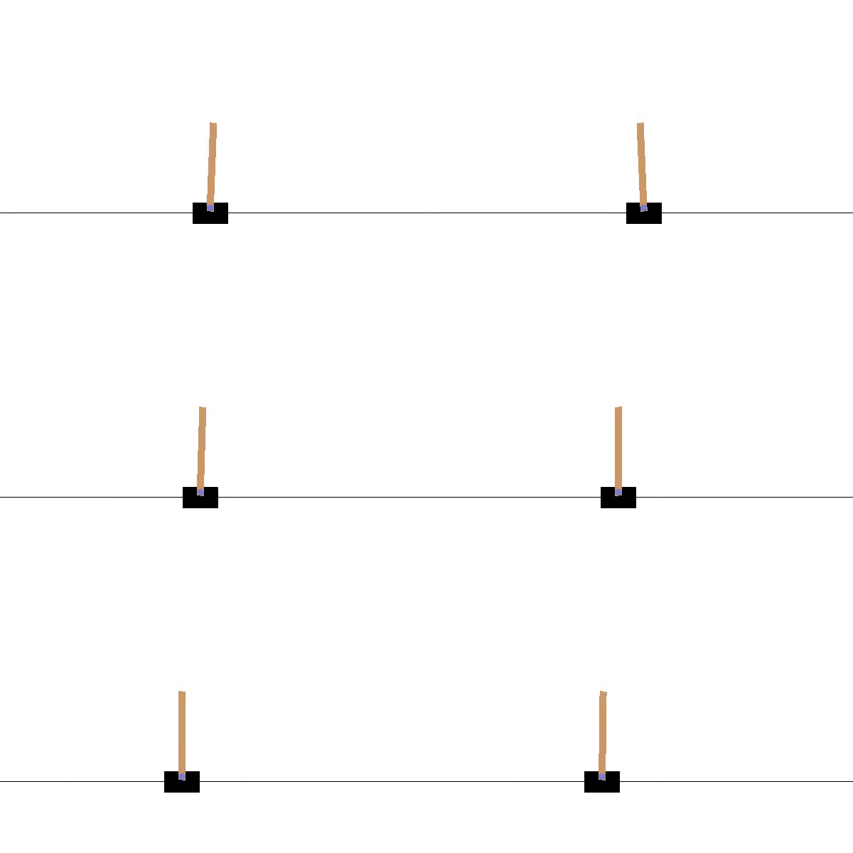
To serve as our expert, we have trained a simple feedforward neural network with architecture (4, 24, 24, 2). It always keeps the pole perfectly upright, reaching the maximum reward of 500 on every episode.
The neural network implementation is below.
class MLPAgent:
    def __init__(self, exploration_rate=EXPLORATION_MAX):
        self.exploration_rate = exploration_rate
        self.memory = deque(maxlen=MEMORY_SIZE)

        self.model = Sequential()
        self.model.add(Dense(24, input_shape=(4,), activation="relu"))
        self.model.add(Dense(24, activation="relu"))
        self.model.add(Dense(2, activation="linear"))
        self.model.compile(loss="mse", optimizer=Adam(lr=ALPHA))

    def predict(self, state):
        s = np.reshape(state, (1, 4))
        return self.model.predict(s)[0]

    def batch_predict(self, X):
        X = np.reshape(X, (len(X), 4))
        return self.model.predict(X)

    def fit(self, state, target):
        s = np.reshape(state, (1, 4))
        t = np.reshape(target, (1, 2))
        self.model.fit(s, t, verbose=0)

    def batch_fit(self, X, y):
        self.model.fit(X, y, verbose=0)

    def act(self, state):
        if np.random.rand() < self.exploration_rate:
            return random.randrange(2)
        q_values = self.predict(state)
        return np.argmax(q_values)

    def remember(self, state, action, reward, next_state, done):
        self.memory.append((state, action, reward, next_state, done))

    def experience_replay(self):
        if len(self.memory) < BATCH_SIZE:
            return

        X = []
        y = []

        batch = random.sample(self.memory, BATCH_SIZE)

        for state, action, reward, next_state, done in batch:
            if done:
                target_q = reward
            else:
                target_q = reward + GAMMA * np.amax(self.predict(next_state))

            target = self.predict(state)
            target[action] = target_q

            X.append(state)
            y.append(target)

        X = np.array(X)
        y = np.array(y)

        self.batch_fit(X, y)

        self.exploration_rate *= EXPLORATION_DECAY
        self.exploration_rate = max(EXPLORATION_MIN, self.exploration_rate)

    def save_model(self, filename):
        self.model.save(filename)

    def load_model(self, filename):
        self.model = keras.models.load_model(filename)
Behavior Cloning
As previously stated, the goal of Imitation Learning is to create an agent (called the student) that mimics another - ideally optimal - agent (called the expert). In RL lingo, this means that we have an expert policy $\pi^{*}$, and we want to obtain a policy $\pi$ that approximates it.
The most intuitive approach possible (which is something that might have already crossed your mind) is to reduce this problem to Supervised Learning:
- Let the expert policy $\pi^{*}$ interact with the environment.
- Collect the data from the expert interaction, generating a dataset $D = {(s_{\sim \pi^{*}}, \pi^{*}(s))}$.
- Run the Supervised Learning algorithm of your choice on the dataset $D$.
Since the supervised model is trained to receive a state $s$ and predict an action $a = \pi^*(s)$, it effectively corresponds to the student policy $\pi$ that was desired. Bam!
This approach is called behavior cloning (BC), and what I like about it is the simplicity: it’s the first thing you’d think of, and it actually works. No Q-values, no value updates, nothing - just plain old supervised learning. Let’s see this approach in action.
Implementation
The code for our implementation of behavior cloning is included below. We collected 100 episodes from the expert (i.e. 50000 pairs $(\text{state}, \text{action})$), and used the decision tree CART algorithm as our supervised model (in particular, its implementation in scikit as the DecisionTreeClassifier model). Using a pruning parameter of $\alpha = 0.02$, the tree obtained by Behavior Cloning was:
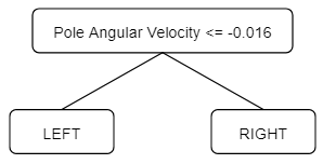
We can easily interpret what it’s doing: if the pole is actively falling to the left, then move the cart to the left, and if the pole is falling to the right then move the cart to the right as well.
This tree has a mean reward of 191.46 ± 65.36, measured over 100 episodes. The obtained reward isn’t bad (a random policy would obtain a mean reward of ~10), but it is far from the consistent +500 obtained by the expert neural network. In other words, there’s definitely some room for improvement here.
Code
import gym
import numpy as np
from sklearn import tree
import ann

def get_dataset_from_model(config, model, episodes, verbose=False):
    env = gym.make(config["name"])

    X = []
    y = []

    for _ in range(episodes):
        state = env.reset()
        done = False

        while not done:
            action = model.act(state)
            next_state, _, done, _ = env.step(action)

            X.append(state)
            y.append(action)

            state = next_state

    env.close()

    X = np.array(X)
    y = np.array(y)

    return X, y

if __name__ == "__main__":
    config = {
        "name": "CartPole-v1",
        "can_render": True,
        "episode_max_score": 195,
        "should_force_episode_termination_score": True,
        "episode_termination_score": 0,
        "n_actions": 2,
        "actions": ["left", "right"],
        "n_attributes": 4,
        "attributes": [
            ("Cart Position", "continuous", -1, -1),
            ("Cart Velocity", "continuous", -1, -1),
            ("Pole Angle", "continuous", -1, -1),
            ("Pole Angular Velocity", "continuous", -1, -1)],
    }

    # Get expert from another file
    expert = ann.MLPAgent(config, exploration_rate=0)
    expert.load("data/cartpole_nn_expert")

    # Create D
    X, y = get_dataset_from_model(config, expert, episodes=100)

    # Fit supervised model
    dt = tree.DecisionTreeClassifier(ccp_alpha=0.01)
    dt.fit(X, y)
Disadvantages
Although the above example may not make this clear, there is a crucial problem in the BC approach: the input distributions are inherently different in the training and test phases.
- Suppose you have trained a student policy $\pi$ to imitate the expert $\pi^{*}$, such that the imitation isn’t perfect (i.e. $\pi(s) \neq \pi^{*}(s)$ for some state $s$)
- Since $\pi$ is not a perfect copy of $\pi^{*}$, it may sometimes take actions that the expert would not have taken.
- Therefore, the student $\pi$ can end up in situations which the expert $\pi^{*}$ would have avoided.
This is a problem!
- Since the expert would have avoided these situations, there is no record of them in the dataset $D$ used to obtain $\pi$.
- Therefore, the student $\pi$ doesn’t have a good example of how to react in this situation.
The usual example given here is enlightening: think of a car racing game. It’s entirely plausible that the student $\pi$, by virtue of being an imperfect copy of the expert $\pi^{*}$, may end up close to the edge of the track - where a crash is imminent, but avoidable. Since the expert $\pi^{*}$ usually sticks to the middle of the road, there is no example of “avoiding edge crashes” in the dataset $D$ used to obtain $\pi$ - the expert $\pi^{*}$ wouldn’t have been in the edge in the first place! Therefore, the student doesn’t have any idea of what the expert would to in this scenario - a bad situation just became worse.
In behavior cloning, errors accumulate.
In more technical terms, the problem is that your supervised model faces different distributions during training and testing: you’ll train the policy $\pi$ based on data collected from $\pi^{*}$, but you’ll test the policy $\pi$ on data collected from... itself, because it won’t have the expert at test time. This is called covariate shift, and although it isn’t always be a problem, it’s definitely something to keep in mind. (Note that if you can perfectly mimic $\pi^{*}$, then the distributions are the same and you won’t have this problem).
So in conclusion, behavior cloning is very simple and may work in some situations, but stay alert: if your student policy is prone to occasional horrible performances, you already know what’s up.
Alternating Optimization
Upon hearing the disadvantages of behavior cloning, something may have crossed your mind: “well, if the problem is that we’re training and testing using different policies, then what if the states in the dataset were not sampled by the expert, but only labeled by it?”. The resulting algorithm would go something like this:
- Generate an initial student policy $\pi_0$ (e.g. using behavior cloning).
- Initialize $i \leftarrow 0$
- Let the student policy $\pi_i$ interact with the environment.
- Use the expert $\pi^{*}$ to label each state $s$ visited by $\pi_i$, generating dataset $D = {(s_{\sim \pi_i}, \pi^{*}(s))}$.
- Run the Supervised Learning algorithm of your choice on the dataset $D$.
- The trained supervised model corresponds to the new policy $\pi_{i+1}$.
- Update $i \leftarrow i + 1$
- Return to step 3.
In other words, the idea here is that the student provides the state distribution, while the expert provides the correct actions. This approach avoids the main issue of behavior cloning because now we’re training and testing on the same state distribution, extracted from the student policies $\pi$. In other words, if the student $\pi$ ends up in the edge of the road during testing, then it will know how the expert would react in this situation, because this same situation would have been brought up during step 3 of the algorithm above, and the expert reaction would already be included in the dataset $D$!
This approach is called alternating optimization (AO) by Yisong Yue and Hoang Le in their ICML 2018 workshop on Imitation Learning[^1]. Let’s see this approach in action.
Implementation
We ran 50 iterations of alternating optimization, with dataset containing 200 episodes. Similarly to the previous BC example, we employed a pruning parameter of $\alpha = 0.02$. The results are plotted in the following graph:
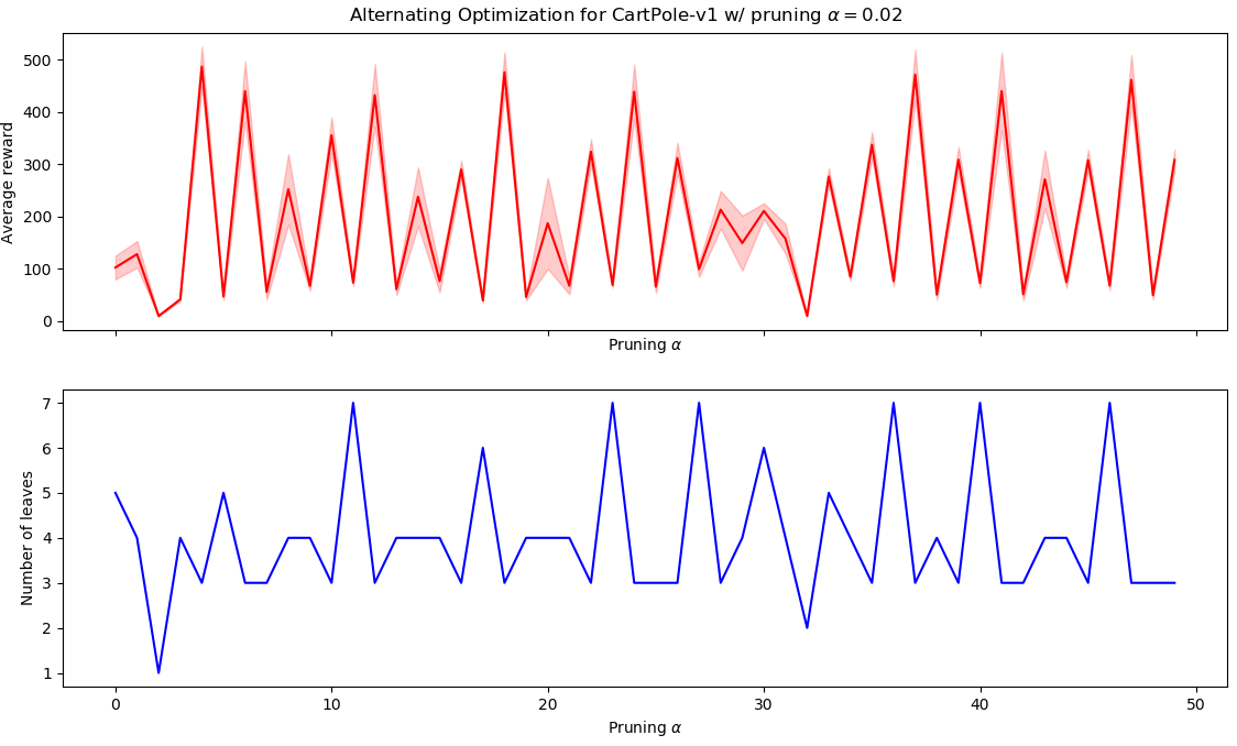
As we can see, the algorithm consistently alternates between good and bad policies in a very periodic manner. The best policy was obtained in iteration ~5, and corresponds to the following tree:
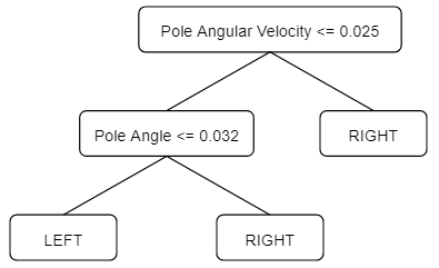
The average reward for this tree is whopping 465.79 ± 80.97, greatly surpassing the 191.46 ± 65.36 obtained in the BC approach! This result is all the more interesting because the tree is still very interpretable: the cart only moves left if pole angle ≤ 0.032 and pole angular velocity ≤ 0.25, that is, if the pole is tilted to the left and is falling to the left. differs from the best BC tree by only one additional split.
Code
import ann

import gym
import numpy as np
from sklearn import tree

def get_dataset_from_model(config, model, episodes, verbose=False):
    env = gym.make(config["name"])

    X = []
    y = []

    for _ in range(episodes):
        state = env.reset()
        done = False

        while not done:
            action = model.act(state)
            next_state, _, done, _ = env.step(action)

            X.append(state)
            y.append(action)

            state = next_state

    env.close()

    X = np.array(X)
    y = np.array(y)

    return X, y

def label_dataset_with_model(config, model, X):
    y = model.batch_predict(X)
    y = [np.argmax(q) for q in y]
    return y

if __name__ == "__main__":
    config = {
        "name": "CartPole-v1",
        "can_render": True,
        "episode_max_score": 195,
        "should_force_episode_termination_score": True,
        "episode_termination_score": 0,
        "n_actions": 2,
        "actions": ["left", "right"],
        "n_attributes": 4,
        "attributes": [
            ("Cart Position", "continuous", -1, -1),
            ("Cart Velocity", "continuous", -1, -1),
            ("Pole Angle", "continuous", -1, -1),
            ("Pole Angular Velocity", "continuous", -1, -1)],
    }

    # Get expert from another file
    expert = ann.MLPAgent(config, exploration_rate=0)
    expert.load("data/cartpole_nn_expert")

    # Initialize dataset and policy
    X, y = get_dataset_from_model(config, expert, episodes=100)
    dt = tree.DecisionTreeClassifier(ccp_alpha=0.01)
    dt.fit(X, y)

    best_reward = -np.inf
    best_model = None

    for i in range(50):
        # Get D'
        X, _ = get_dataset_from_model(config, dt, episodes=100)
        y = label_dataset_with_model(config, expert, X)

        # Update student policy pi_i
        dt = tree.DecisionTreeClassifier(ccp_alpha=0.01)
        dt.fit(X, y)

        # Evaluate average reward from student policy pi_i
        avg_reward = get_average_reward(config, dt) # Function not pictured here

        # Keep tabs on best policy seen so far
        if avg_reward > best_reward:
            best_reward = avg_reward
            best_model = dt
Disadvantages
Sadly, there is a crucial problem to AO: it doesn’t have any convergence guarantees. Since this is the case, there’s nothing stopping the algorithm from e.g. alternating between two different policies. In fact, we can hypothesize a situation in which this two-policy-hopping could arise:
- $\pi_1$ is a close-to-optimal policy, i.e. $\pi_1 \approx \pi^*$.
- Since $\pi_1$ is good at what it does, the data collected by it rarely contains any “low-reward” states. Example: the car always sticks to the middle of the road.
- Any policy $\pi_2$ learned by fitting the dataset $D_1 = {(s_{\sim \pi_1}, \pi^{*}(s))}$ is possibly low-quality, since it faces the same issue described in the “behavior cloning” section: $\pi_2$ may not know what to do to correct a mistake. Therefore, $\pi_2$ is a bad policy.
- $\pi_2$ is a bad, effectively random policy.
- $\pi_2$ can be bad in a way that is effectively random. Therefore, it visits tons of states during its data collection phase. Example: the car goes all over the road.
- Since different states are visited, the dataset $D_2 = {(s_{\sim \pi_2}, \pi^{*}(s))}$ has a more diverse input distribution, all of them with correct labels. If a policy $\pi_3$ is fitted on $D_2$, there’s a chance that it would be way better than $\pi_2$. Therefore, $\pi_3$ is plausibly a good, close-to-optimal policy, similar to $\pi_1$.
- Therefore, the algorithm can alternate between good and bad policies.
As far as I know, this explains the jagged alternations in the CartPole results above: the algorithm is alternating between good and bad policies. Stated another way, this happens because Alternating Optimization can easily forget the lessons learned: a pair $(\text{state},\text{correction})$ only lasts for a single iteration, therefore hopping may occur. As we will see, the third and last algorithm avoids this problem by design.
DAgger (Dataset Aggregation)
DAgger picks up just where AO left off; it avoids forgetting previous errors by, as it name implies, aggregating datasets. The algorithm could be described this way:
- Generate an initial student policy $\pi_0$ (e.g. using behavior cloning).
- Initialize $i \leftarrow 0$
- Let the student policy $\pi_i$ interact with the environment.
- Use the expert $\pi^{*}$ to label each state $s$ visited by $\pi_i$, generating a dataset $D' = {(s_{\sim \pi_i}, \pi^{*}(s))}$.
- Aggregate the new dataset $D'$ with all previously-seen datasets: $D \leftarrow D' \cup D$
- Run the Supervised Learning algorithm of your choice on the aggregated dataset $D$.
- The trained supervised model corresponds to the new policy $\pi_{i+1}$.
- Update $i \leftarrow i + 1$
- Return to step 3.
As we can see, the algorithm is really just aggregating datasets and creating an ever-increasing storage of previous experiences and corrections. This avoids the problem of forgetting because nothing is forgotten - it all just gets aggregated into a giant dataset. Alternating between policies also diminishes because the policy $\pi_i$ has access to whatever data $\pi_{i-1}$ had access to, therefore the situation described inthe previous section wouldn’t happen.
(It’s also worth pointing out that, in DAgger’s original paper [^2], the authors additionally proposed to mix student and expert policies when collecting the dataset $D'$. This seems to be particularly useful in the first iterations, when student policies are bad. We did not take this approach, since it appeared to be unnecessary in a simple task such as CartPole).
Let’s see DAgger in action.
Implementation
We ran DAgger using the same parameters as the previous alternating optimization: 50 iterations with 200 episodes each, and pruning level of $\alpha = 0.02$. This produced the following graph:
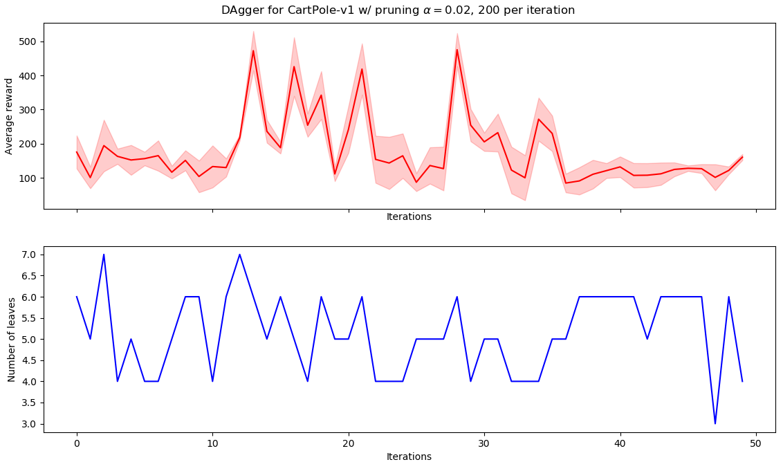
As we can see, there is no hopping between different policies (as AO did), although there is no convergence as well. This is fine, since the guarantee provided by DAgger is not that the algorithm converges to a good policy, but merely that it finds a good policy sometime during its execution. (By “good”, we mean within a certain distance of the optimal. For more details check the paper).
The following tree reaches the maximum average reward of 458.26 ± 89.16:
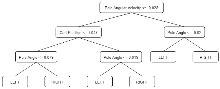
As we can see, the tree is larger than the one found by AO, while having comparable performance. This is possibly due to dataset size: since DAgger aggregates datasets, CART has more data; consequently, it needs a higher number of nodes to fit adequately to this larger dataset. This would usually be a good thing, since fewer data is closely related with overfitting, however CartPole is such a simple environment that this appears to be overkill.
Therefore, in this particular case, DAgger appear to be superseded by the simpler AO.
Code
import ann

import gym
import numpy as np
from sklearn import tree

def get_dataset_from_model(config, model, episodes, verbose=False):
    env = gym.make(config["name"])

    X = []
    y = []

    for _ in range(episodes):
        state = env.reset()
        done = False

        while not done:
            action = model.act(state)
            next_state, _, done, _ = env.step(action)

            X.append(state)
            y.append(action)

            state = next_state

    env.close()

    X = np.array(X)
    y = np.array(y)

    return X, y

def label_dataset_with_model(config, model, X):
    y = model.batch_predict(X)
    y = [np.argmax(q) for q in y]
    return y

if __name__ == "__main__":
    config = {
        "name": "CartPole-v1",
        "can_render": True,
        "episode_max_score": 195,
        "should_force_episode_termination_score": True,
        "episode_termination_score": 0,
        "n_actions": 2,
        "actions": ["left", "right"],
        "n_attributes": 4,
        "attributes": [
            ("Cart Position", "continuous", -1, -1),
            ("Cart Velocity", "continuous", -1, -1),
            ("Pole Angle", "continuous", -1, -1),
            ("Pole Angular Velocity", "continuous", -1, -1)],
    }

    # Get expert from another file
    expert = ann.MLPAgent(config, exploration_rate=0)
    expert.load("data/cartpole_nn_expert")

    # Initialize dataset and policy
    X, y = get_dataset_from_model(config, expert, episodes=100)
    dt = tree.DecisionTreeClassifier(ccp_alpha=0.01)
    dt.fit(X, y)

    best_reward = -np.inf
    best_model = None

    for i in range(50):
        # Get D'
        X2, _ = get_dataset_from_model(config, dt, 100)
        y2 = label_dataset_with_model(config, expert, X2)

        # Aggregate datasets
        X = np.concatenate((X, X2))
        y = np.concatenate((y, y2))

        # Update student policy pi_i
        dt = tree.DecisionTreeClassifier(ccp_alpha=0.01)
        dt.fit(X, y)

        # Evaluate average reward from student policy pi_i
        avg_reward = get_average_reward(config, dt) # Function not pictured here

        # Keep tabs on best policy seen so far
        if avg_reward > best_reward:
            best_reward = avg_reward
            best_model = dt
Disadvantages
Although DAgger is the most popular active imitation learning algorithm, it also comes with its own noteworthy disadvantages:
- It starts not-so-great. On the first iterations, it’s possible that the student policies have low-quality behavior. This may be undesirable in some situations (e.g. you never want your robot to fall over, or your autonomous driver to crash, etc).
- It requires an interactive expert. As an active imitation learning algorithm, DAgger requires that you have an expert available to provide feedback on the student’s mistakes; however, sometimes you just have a dataset of expert interactions, and that’s it! In these scenarios, DAgger is not applicable.
- It may be equal or worse than behavior cloning. As we noted in our AO-DAgger comparison, DAgger is not always the best choice. From this BAIR Blog post[^3]: “If the [student] is able to learn the [expert]’s policy perfectly, then it should visit the same states as the [expert]. In prior work we empirically found in simulation that with sufficient data and expressive learners, such as deep neural networks, Behavior Cloning is at parity with DAgger”.
Conclusion
In this post we explored three popular active imitation learning algorithms, and we have also seen how they are built on top of one another. I have also provided implementations for all three on the CartPole environment, and we have seen that DAgger truly appears to be the best among them.
If you find a mistake in this post, please leave a comment or contact me via e-mail! I am Learning in Public, so mistakes will be made. Nevertheless, I hope this helps you in some way :)
Resources
[^1] “Imitation Learning Tutorial ICML 2018”, by Yisong Yue and Hoang M. Le [^2] “A Reduction of Imitation Learning and Structured Prediction to No-Regret Online Learning”, by Ross et al. (2011)- The original DAgger paper.
- https://www.ri.cmu.edu/pub_files/2011/4/Ross-AISTATS11-NoRegret.pdf
- BAIR blog post about DART.
- https://bair.berkeley.edu/blog/2017/10/26/dart/
Web tool used for drawing the trees: link.
